Your brain just processed this sentence.
You were able to do it completely subconsciously, but most modern LLMs individually process each word: one at a time, weighing their relationships, and extracting meaning in parallel.
Today, Anthropic's Claude writes production-ready code. Google's Aeneas translates ancient languages. GPT-4 passes the bar exam. How does a machine essentially made of sand and rocks understand language well enough to do these things?
Before 2017, building a model that understood context meant accepting fundamental tradeoffs. You could have speed or memory of distant words, but not both. The Transformer changed that equation entirely. And it started with one question: what if a model could look at all the words at the same time?
The Sequential Processing Bottleneck
Before Transformers, language models processed text sequentially using RNNs (Recurrent Neural Networks) and LSTMs (Long Short-Term Memory networks).
Think about reading this sentence: "The cat, which had been sleeping on the warm sunny windowsill for hours, finally woke up."
An RNN processes it like this:
# Simplified RNN pseudocode showing the sequential bottleneck
hidden_state = initial_state

for word in sentence:
    hidden_state = rnn_cell(word, hidden_state)
    # Must wait for previous word to complete!
    # for example "finally" can't be processed until it's done with all prev words
The RNN has to process "The", then "cat", then "which", and so on. By the time it reaches "finally", the information about "cat" has been compressed through 10+ sequential operations. This creates two major problems:
The vanishing gradient problem: As info passes through many sequential steps, the gradient signal that helps the model learn gets weaker and weaker. Hochreiter & Schmidhuber (1997) showed that RNNs struggle to learn dependencies that span more than a few steps.
No parallelization: You can't process word 10 until you've processed words 1-9. This makes training painfully slow.
LSTMs improved on basic RNNs by adding a "memory cell" that could preserve information longer, but still processed information sequentially. They were SOTA for nearly two decades, but the fundamental bottleneck remained.1
The Birth of Attention
In 2014, Bahdanau et al. introduced attention mechanisms for machine translation. What if, when translating a word, the model could "look at" all the source words, not just a compressed "hidden state"? Instead of forcing all "context" through a sequential bottleneck, attention lets the model directly access any word it needed.
But this attention was still being used alongside RNNs. The real breakthrough came in 2017 when team at Google asked: what if we removed the recurrence entirely?
Their paper, "Attention is All You Need", introduced the Transformer architecture. No RNNs. No LSTMs. Just attention (source and self), feed-forward layers, and some clever positional encoding.
On the WMT 2014 English-to-German translation task, their model achieved a BLEU score of 28.4, beating the previous state of the art by over 2 points. On English-to-French, they hit 41.0 BLEU.2 And it trained in a fraction of the time.
Within a few years, Transformers became the foundation for BERT, GPT, and essentially every major language model that followed.
Understanding Attention: The Core Mechanism
Let's build this up from scratch.
The Intuition
When you read "The animal didn't cross the street because it was too tired," your brain automatically knows "it" refers to "animal," not "street." Your brain pays attention to the relevant context.
Attention mechanisms give neural networks this same ability. When processing "it", the model can look back at all previous words and decide which ones matter most.
The model learns to assign high attention weight to "animal" (0.7), medium weights to "didn't" (0.15) and "tired" (0.1), and very low weights to "street" (0.03) and others (0.02).
But how does it actually compute these weights?
The Math: Query, Key, Value
Attention works through three learned transformations of the input:
- Query (Q): "What am I looking for?"
- Key (K): "What do I contain?"
- Value (V): "What information do I actually have?"
This is somewhat analogous to database retrieval. When you query a database, you provide a query that gets matched against keys in the database, and the matching records return their values.
Let's say we have a sentence: "The cat sat". Each word starts as an embedding vector (ie 512 or 768 dimensions). For each one, we create three vectors:
# Each word embedding x gets projected to Q, K, V
Q = x @ W_q  # Query: what should I pay attention to?
K = x @ W_k  # Key: what do I offer to others?
V = x @ W_v  # Value: what information do I carry?
The matrices W_q, W_k, and W_v are learned parameters.
Now we have Q, K, and V vectors for every word. Then we compute attention.
Scaled Dot-Product Attention
The official attention formula is:
Attention(Q, K, V) = softmax(QK^T / √d_k) VLet's break this down step by step with a concrete example: the three-word sentence "The cat sat".
Step 1: Compute attention scores
Take the dot product between every Query and every Key. This tells us how much each word should attend to each other word.
# Q shape: (batch, seq_len, dim) = (1, 3, 64)
# K shape: (batch, seq_len, dim) = (1, 3, 64)
scores = Q @ K.transpose(-2, -1)  # Result: (1, 3, 3)
The result is a 3×3 matrix where entry (i,j) represents how much word i attends to word j.
Step 2: Scale the scores
d_k = Q.size(-1)  # dimension of key vector, e.g., 64
scores = scores / math.sqrt(d_k)  # Divide by √64 = 8
Why scale? Without it, for high-dimensional vectors, dot products can become very large.
Super large values pushed through softmax cause extremely peaked distributions, which makes gradients very small and training difficult.
Step 3: Apply softmax
The Softmax function turns the raw scores into nice probabilities [0, 1] for the model to understand.
attention_weights = F.softmax(scores, dim=-1)
# Each row now sums to 1.0 and represents a prob distribution

# Example: After scaling, scores might look like:
# [[2.1, 0.8, -0.3],   # "The" attending to ["The", "cat", "sat"]
#  [1.2, 3.5,  1.8],   # "cat" attending to ["The", "cat", "sat"]
#  [0.5, 2.1,  2.9]]   # "sat" attending to ["The", "cat", "sat"]

# After softmax, attention_weights become:
# [[0.68, 0.19, 0.13],  # "The" attends mostly to itself
#  [0.09, 0.76, 0.15],  # "cat" attends mostly to itself
#  [0.08, 0.38, 0.54]]  # "sat" attends to "cat" and itself
# Each row sums to 1.0
Step 4: Weighted sum of values
For each word (token), we compute a weighted combination of all the Value vectors, where the weights come from our attention distribution. Each token has a QKV relating it with all other tokens.
This weighted sum creates a context-aware representation for each token. Instead of "it" being just a generic pronoun embedding, it becomes "it-in-the-context-of-animal-being-tired" by pulling relevant information from other tokens.
This output gets passed to the next layer, which builds even richer representations through more rounds of attention. This is the heart of the Transformer. Everything else builds on the attention mechanism.
Multi-Head Attention: Learning Different Patterns
A single attention mechanism is powerful, but it can only learn one type of relationship at a time. What if different parts of the model could learn different patterns?
Multi-head attention runs multiple attention mechanisms in parallel, each with different queries learning different aspects of the relationships between words:
- Head 1 might learn syntactic relationships (subject-verb, adjective-noun)
- Head 2 might learn semantic relationships (synonyms, antonyms)
- Head 3 might focus on positional relationships (adjacent words)
- Head 4 might capture long-range dependencies
The Architecture
Multi-head attention divides the input embedding into h heads. Each head performs scaled dot-product attention independently. The outputs are then concatenated and passed through a final linear transformation.
If our base model dimension is 512 and we have 8 heads, each head works with 512/8 = 64 dimensions.
The best part? All attention heads can be computed in parallel. Because the dimension is split across heads (d_model/h per head), you get multiple attention patterns for the same computational cost as single-head attention with the full dimension.
Positional Encoding: How the model understands ordering
Attention is permutation-invariant. The sentences "The cat sat on the mat" and "mat the on sat cat The" would produce identical outputs. Attention has no understanding of word order.3
If you've made it this far, you should understand that order matters in language. "Dog bites man" means something very different from "Man bites dog."
The proposed solution: positional encoding. Before feeding word embeddings into the transformer, we inject position information to each embedding.
Sinusoidal Positional Encoding
The original Transformer paper uses sinusoidal functions to encode position:
PE(pos, 2i) = sin(pos / 10000^(2i/d_model))
PE(pos, 2i+1) = cos(pos / 10000^(2i/d_model))
Where:
posis the position (0, 1, 2, ...)iis the dimension index (0, 1, 2, ..., d_model/2)- Even dimensions use sine, odd dimensions use cosine
Why sinusoids?
- Unique encoding: Each position gets a unique encoding pattern
- Relative positions: The model can learn to attend to relative positions (e.g., "attend to the word 3 positions back")
- Bounded extrapolation: Theoretically works for arbitrary positions, though in practice models struggle with lengths much longer than training data—a limitation that drove development of RoPE, ALiBi, and other improved schemes
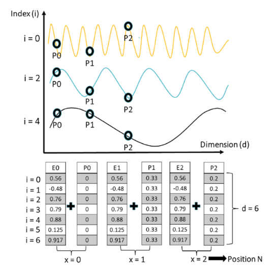
This encoding strategy is actually super similar to binary encoding.
The positional encoding is added to the word embedding, not concatenated. This means position information is mixed directly into the representation that attention operates on.
Different positions create wave patterns at different frequencies. Low-frequency waves change slowly (capturing global position), while high-frequency waves change quickly (capturing local position).
The Complete Transformer
Now we have all the pieces. Let's assemble them into the full architecture.
The Transformer has an encoder-decoder structure.4 The encoder processes the input sequence (like an English sentence), building a rich contextual understanding. The decoder then generates the output sequence (like a French translation), attending back to the encoder's representations while producing tokens one at a time.
Encoder
Each encoder layer has two sublayers:
- Multi-head self-attention: Allows each word to attend to all other words in the input
- Feed-forward network: Two linear layers with ReLU activation
Both sublayers use residual connections and layer normalization:
output = LayerNorm(x + Sublayer(x)) # this is a residualThis helps training by allowing gradients to flow directly through the network. The encoder stack has N=6 identical layers, so the input passes through 6 rounds of self-attention and feed-forward processing.
Decoder
The decoder is more complex. Each decoder layer has three sublayers:
- Masked multi-head self-attention: Prevents positions from attending to future positions
- Multi-head cross-attention: Attends to the encoder's output
- Feed-forward network: Same as in the encoder
The key difference is token masking. During training, we have the complete target sequence, but we can't let position i see positions beyond i (that would be cheating). During inference, we generate one token at a time anyway.
def create_causal_mask(size):
    """
    Create a mask that prevents attending to future positions.
    Returns a lower-triangular matrix of True values.
    """
    mask = torch.triu(torch.ones(size, size), diagonal=1)
    return mask == 0  # Lower triangle = True (visible)
The decoder uses the same residual connections and layer normalization as the encoder, with 6 identical layers processing the target sequence while attending to both previous target tokens and the full encoder output.
Why Transformers Won
Transformers process all tokens in parallel. While RNNs require O(n) sequential steps to connect distant tokens, Transformers connect any two tokens through a single attention operation—O(1) path length. The computational cost is O(n²) due to the attention matrix, but this parallelizes efficiently on modern GPUs.
On modern chips optimized for parallel computation, this translates to 10-100× faster training on the same data. Long-range dependencies that plagued RNNs become trivial. Connecting tokens 100 steps apart no longer requires information to flow through 100 sequential operations, degrading with each step. In a Transformer, any two tokens connect through a single attention operation. The model can directly reference a word from the beginning of a paragraph when processing the end.
Bigger models trained on more data consistently perform better, following predictable scaling laws. There's no architectural ceiling. Add more layers, more heads, more parameters, and performance improves.
This scaling property enabled the jump from BERT (340M parameters) to GPT-3 (175B) to GPT-4. Combined with transfer learning, where you pre-train once on massive unlabeled data then fine-tune for specific tasks, the paradigm shifted entirely. By 2020, you didn't even need fine-tuning; just describe the task in a prompt and get results.
| Property | RNN | LSTM | Transformer |
|---|---|---|---|
| Sequential depth | O(n) | O(n) | O(1) |
| Max path length | O(n) | O(n) | O(1) |
| Parallelizable | No | No | Yes |
| Training speed (relative) | 1× | 1× | 10-100× |
| Long-range deps | Poor | Moderate | Excellent |
The difference in training speed is dramatic. On modern hardware (GPUs/TPUs), Transformers train 10-100× faster than RNNs on the same data.
State Space Models
In 2023-2024, a new family of architectures emerged called State Space Models (SSMs).
The pitch is compelling: match Transformers' performance while solving the O(n²) attention bottleneck with linear complexity. SSMs process sequences through a compressed hidden state that evolves recurrently, similar to RNNs but with key innovations: larger state size (storing more information), selective state updates (choosing what to remember like LSTM gates), and efficient parallel training algorithms.
Gu (2025) frames the fundamental tradeoff elegantly: SSMs have efficient, stateful processing with compressed representations, while Transformers maintain perfect recall with an explicit token-level cache.
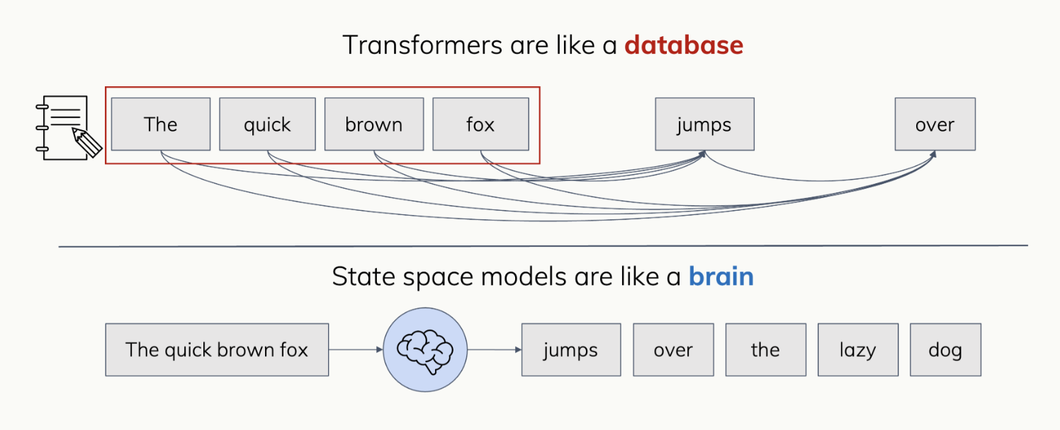
This makes SSMs excel at long-sequence tasks and online processing, but Transformers still dominate on tasks requiring precise retrieval, complex reasoning over context, and in-context learning, the very capabilities that made LLMs transformative.
So why do Transformers still dominate? The answer is both empirical and practical. Transformers remain superior on most language understanding benchmarks, particularly those requiring fine-grained manipulation of context or few-shot learning.
There's also billions of dollars in infrastructure, pre-trained checkpoints, and tooling optimized for Transformers. Can't say the same about any other architecture.
SSMs aren't replacing Transformers; they're pushing the field forward. Hybrid architectures like Jamba combine Transformer layers for reasoning with Mamba layers for efficient long-context processing, suggesting the future may involve using the right tool for each part of the model.
The Bigger Picture
Before 2017, every NLP task required its own model trained from scratch on limited labeled data. Translation needed a translation model, summarization needed a summarization model, sentiment analysis needed yet another model. The Transformer changed that.
Suddenly you could pre-train one massive model on unlabeled text, then fine-tune it for any specific task with minimal data. By the 2020s, even fine-tuning became optional; just describe what you want in natural language and the model does it. Few-shot and zero-shot learning made NLP accessible to anyone who could write a prompt.
The attention mechanism answered a simple question: "what should the model focus on?"
Claude writing code, ChatGPT holding conversations, AlphaFold predicting protein structures, all built on the foundation of attention.
The original Transformer paper has been cited over 100,000 times. It's one of the most influential computer science papers of the 21st century. The eight authors scattered across the industry: Noam Shazeer founded Character.AI (returned to Google in a $2.7B licensing deal), Aidan Gomez founded Cohere, Llion Jones and Niki Parmar joined other AI labs.
But we're still early.
Models are getting larger, more capable, and more generalized. And architectural innovations continue: sparse attention for efficiency, mixture of experts for scale, and so much more.
The question "what should I pay attention to?" turns out to be fundamental to intelligence, both artificial and natural. And we're only just beginning to explore its possibilities.
→ Kyle
Footnotes
- 1.
LSTMs solved some of RNN's problems but not the sequential computation bottleneck. They can remember longer dependencies (100+ steps vs RNN's 10-20), but training is still sequential, making them slow on modern hardware that excels at parallel computation. Here's a great blog about them from Chris Olah (Cofounder of Anthropic) Post here
- 2.
BLEU (Bilingual Evaluation Understudy) is the standard metric for machine translation quality. It measures how many n-grams (1-4 word sequences) in the machine translation match those in reference human translations, with scores from 0-100. A BLEU of 28.4 was groundbreaking in 2017, closer to human-level translation quality (mid-30s) than previous models.
- 3.
This is actually both a bug and a feature. Permutation invariance is useful for some tasks (like processing a set of objects). But for sequences where order matters (language, time series), we need to inject positional information explicitly.
- 4.
Many modern models use only the decoder (GPT series) or only the encoder (BERT). But the original Transformer and many translation models use both. The encoder-decoder split allows the model to first fully understand the input, then generate the output while attending back to that understanding.